Statistical distributions and parameter estimation
Predefined joint models
Predefined joint model structures are available in the module predefined.py.
- Currently, four predefined models are available:
Wind speed – wave height model recommended in DNV’s guideline on environmental conditions [1]
Wind speed – wave height model proposed by Haselsteiner et al. (2020) [2]
Wave height - wave period model recommended in DNV’s guideline on environmental conditions [1]
Wave height - wave period model proposed by Haselsteiner et al. (2020) [2]
Additional model structures can be added to the predefined.py module.
In the documentation’s quick start example section a predefiend wave height - wave period model structure is used.
Custom joint models
In the documentation’s detailed examples section custom joint models are defined and used (instead of predefined models).
Parameter estimation
By default, marginal distribution parameters are estimated using maximum likelihood estimation and dependence function parameters are estimated using least squares, however, other fitting methods can be selected by specifying the “fit_description” dictionary.
The following example shows how first, default parameter estimation used and then weighted least squares is used to estimate the parameter values of the wave height’s distribution.
The code, which is available as a Python file here, will create this plot:
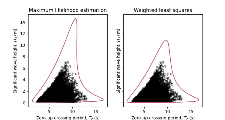
Unless you specify otherwise, the parameters of dependence functions are estimated using weighted least squares.
Implementing new statistical distributions: Example of the generalized gamma distribution
When implementing a new distribution in virocon there are two general approaches available. The first and easiest approach is to use a distribution defined in scipy and directly use it to derive a distribution for virocon (“scipy approach”). A distribution created this way will have the same parameters as the scipy distribution. The second, more flexible approach is to build a new distribution from scratch (“from scratch approach”). Such a distribution may or may not use scipy functions and allows to freely design the distribution parameters. When implementing a new distribution from scratch, we recommend starting with an existing distribution in virocon and adapting it step by step. You can use a virocon distribution as a template to implement a new distribution. The following sections describe how the generalized gamma distribution was implemented (from scratch approach) and how it could have been implemented using the scipy approach.
Scipy approach: Subclassing ScipyDistribution
To create a virocon based on a scipy distribution is as easy as subclassing virocon.distributions.ScipyDistribution
and overwriting one of its attributes: scipy_dist_name or scipy_dist.
Which attribute to overwrite is a matter of preference and does not change the behaviour of the subclass.
The generalized gamma distribution is named ‘gengamma’ in scipy.
from virocon import ScipyDistribution

class GeneralizedGammaDistribution(ScipyDistribution):

    scipy_dist_name = "gengamma"
is equivalent to
from virocon import ScipyDistribution
from scipy.stats import gengamma

class GeneralizedGammaDistributionByDist(ScipyDistribution):

    scipy_dist = gengamma
The resulting distribution class has the same parameters as the scipy distribution: a, c, loc, scale. If instead a 3 parameter version of the distribution is requested, one of the parameters can be fixed creating an instance of the distribution. E.g. fix the location parameter to zero:
my_gengamma = GeneralizedGammaDistributionByDist(f_loc=0)
Second Approach: Building from scratch
If a specific parameterization of the distribution is necessary, or if the distribution to implement is not available in scipy, the distribution can be created from scratch, instead. The steps to create such a distribution is shown in the following with the generalized gamma distribution as an example.
1. Clarify the mathematics of the distribution:
In the following, we implement the 3-parameter generalized gamma distribution as recommended by Ochi (1992) [3]. Its probability density function (PDF) is defined as:
\(f(x)= \frac{c}{\Gamma(m)}\lambda^{cm}x^{cm-1} \exp\left[- (\lambda x)^{c} \right]\)
To implement the generalized gamma distribution, we make use of the functionality of scipy’s implementation of the distribution. Scipy’s implementation is based on the scientific paper of Stacy (1962) [4]. An overview of the generalized gamma distribution is given in [5]. Scipy uses the following PDF:
\(f(x)= \frac{k(x-a)^{kc-1}}{b^{kc}\Gamma(c)} \exp \bigg[- \bigg(\frac{x-a}{b}\bigg)^{k}\bigg]\)
Stacy’s generalized gamma distribution involves 4 parameters. Two shape parameters (k, c), one scale (b) and one location parameter (a). Note that Ochi’s and Stacy’s formulas for the generalized gamma distribution differ. Hence, to use scipy’s functionality, we must convert the individual parameters. Comparing the parameters, it is seen, that:
c=k ,
m=c ,
a=0 , and
λ=1/b
Here, the two shape parameters can be implemented using scipy’s shape parameters. The location parameter will be set to the fixed value zero and the scale parameter needs to be converted and inverted.
2. Define the characteristics of the distribution and implement it step by step:
To implement a new distribution, the new distribution class - in our case the GammaDistribution class - should inherit from the Distribution class in distributions.py.
This init method is called when an object of the class GammaDistribution is created. When a new gamma distribution object is created, we want to make sure that the attributes of the distribution are passed. Therefore, we build a custom constructor, where all parameters of the distribution are initialized with a default value.
def __init__(self, m=1, c=1, lambda_=1, f_m=None, f_c=None, f_lambda_=None):
 self.m = m  # shape
 self.c = c  # shape
 self.lambda_ = lambda_  # reciprocal scale
 self.f_m = f_m
 self.f_c = f_c
 self.f_lambda_ = f_lambda_
When fitting a distribution function, we want to be able to call the parameters. In virocon, this is ensured by “property functions”. A property of an object in Python is a method that seems like a regular attribute to the user (i.e. we can use obj.property instead of obj.property() ).
Since scipy uses a slightly different parametrization, than we do here, we need to convert the scale parameter between these two parametrizations. For this purpose, we define the scipy scale as a property. This allows to calculate the scipy _scale on the fly, using our value of lambda_. With the first method we define scale as a property, that we can call as x=obj._scale . With the second method, we allow to set the “value” of _scale. (obj._scale = x ) , though again we do not store the value directly but instead modify lambda_ accordingly.
@property
def parameters(self):
    return {"m": self.m, "c": self.c, "lambda_": self.lambda_}

@property
def _scale(self):
    return 1 / (self.lambda_)

@_scale.setter
def _scale(self, val):
    self.lambda_ = 1 / val
Here, we convert our parameters to the format scipy understands. It allows to pass values to convert, but if they are None, it uses the distribution instance’s current values instead.
def _get_scipy_parameters(self, m, c, lambda_):
    if m is None:
        m = self.m
    if c is None:
        c = self.c
    if lambda_ is None:
        scipy_scale = self._scale
    else:
        scipy_scale = 1 / lambda_
    return m, c, 0, scipy_scale  # shape1, shape2, location=0, reciprocal scale
The key functions used to describe statistical distributions are the CDF, ICDF and PDF. Therefore, these functions are implemented using scipy’s functions.
def cdf(self, x, m=None, c=None, lambda_=None):
    """
    Cumulative distribution function.

    Parameters
    ----------
    x : array_like,
        Points at which the cdf is evaluated.
        Shape: 1-dimensional.
    m : float, optional
        First shape parameter. Defaults to self.m.
    c : float, optional
        The second shape parameter. Defaults to self.c.
    lambda_: float, optional
        The reciprocal scale parameter . Defaults to self.lambda_.

    """

    scipy_par = self._get_scipy_parameters(m, c, lambda_)
    return sts.gengamma.cdf(x, *scipy_par)

def icdf(self, prob, m=None, c=None, lambda_=None):
    """
    Inverse cumulative distribution function.

    Parameters
    ----------
    prob : array_like
        Probabilities for which the i_cdf is evaluated.
        Shape: 1-dimensional
    m : float, optional
        First shape parameter. Defaults to self.m.
    c : float, optional
        The second shape parameter. Defaults to self.c.
    lambda_: float, optional
        The reciprocal scale parameter . Defaults to self.lambda_.

    """

    scipy_par = self._get_scipy_parameters(m, c, lambda_)
    return sts.gengamma.ppf(prob, *scipy_par)

def pdf(self, x, m=None, c=None, lambda_=None):
    """
    Probability density function.

    Parameters
    ----------
    x : array_like,
        Points at which the pdf is evaluated.
        Shape: 1-dimensional.
    m : float, optional
        First shape parameter. Defaults to self.m.
    c : float, optional
        The second shape parameter. Defaults to self.k.
    lambda_: float, optional
        The reciprocal scale parameter . Defaults to self.lambda_.

    """

    scipy_par = self._get_scipy_parameters(m, c, lambda_)
    return sts.gengamma.pdf(x, *scipy_par)
Another important function is to draw random samples from the distribution. Hence, every statistical function in virocon must provide a draw_sample function:
def draw_sample(self, n, m=None, c=None, lambda_=None):
    scipy_par = self._get_scipy_parameters(m, c, lambda_)
    rvs_size = self._get_rvs_size(n, scipy_par)
    return sts.gengamma.rvs(*scipy_par, size=rvs_size)
Given a data set is available, a user might want to fit a generalized gamma distribution to these data. The fit() method does not provide a return value, instead it sets the instance’s values. The default estimation method is maximum likelihood estimation (MLE), which is why in virocon all statistical distributions are equipped with a function to fit a distribution to a data set by means of the MLE. The user does not pass in keywords arguments here. If a user wants to fix values, they need to pass them to the constructor (__init__).
def _fit_mle(self, sample):
    p0 = {"m": self.m, "c": self.c, "scale": self._scale}

    fparams = {"floc": 0}

    if self.f_m is not None:
        fparams["fshape1"] = self.f_m
    if self.f_c is not None:
        fparams["fshape2"] = self.f_c
    if self.f_lambda_ is not None:
        fparams["fscale"] = 1 / (self.f_lambda_)

    self.m, self.c, _, self._scale = sts.gengamma.fit(
        sample, p0["m"], p0["c"], scale=p0["scale"], **fparams
    )

def _fit_lsq(self, data, weights):
    raise NotImplementedError()
3. Use new distribution:
The above-described steps can be implemented in the distributions.py file of virocon. However, any other file is valid as well. It’s just that the base class Distribution is defined in distributions.py. (If one uses another file it is necessary to import it). The following describes how to add the distribution to virocon, which is entirely optional. In order to use the new implemented distribution, add the name of the new distribution into the variable _all_=[] below the imports.
import math
import copy

import numpy as np
import scipy.stats as sts

from abc import ABC, abstractmethod
from scipy.optimize import fmin

__all__ = [
    "WeibullDistribution",
    "LogNormalDistribution",
    "NormalDistribution",
    "ExponentiatedWeibullDistribution",
    "GeneralizedGammaDistribution",
]
4. Write automatic tests:
Before implementing the new distributions in virocon, we want to know, if the above-described steps and functions really perform as expected. Therefore, the most accurate test is to reconstruct a distribution from literature and compare the results. If the results match, we can have high certainty that we implemented the new distribution correctly. In general, every function of a class should be tested. To conduct automatic tests, virocon uses pytest. To be able to execute these tests automatically, the added test files for a new distribution must be attached to the file test_distributions.py.
def test_generalized_gamma_reproduce_Ochi_CDF():
    """
    Test reproducing the fitting of Ochi (1992) and compare it to
    virocons implementation of the generalized gamma distribution. The results
    should be the same.
    """

    # Define dist with parameters from the distribution of Fig. 4b in
    # M.K. Ochi, New approach for estimating the severest sea state from
    # statistical data , Coast. Eng. Chapter 38 (1992)
    # pp. 512-525.

    dist = GeneralizedGammaDistribution(1.60, 0.98, 1.37)

    # CDF(0.5) should be roughly 0.21, see Fig. 4b
    # CDF(1) should be roughly 0.55, see Fig. 4b
    # CDF(1.5) should be roughly 0.70, see Fig. 4b
    # CDF(2) should be roughly 0.83, see Fig. 4b
    # CDF(4) should be roughly 0.98, see Fig. 4b
    # CDF(6) should be roughly 0.995, see Fig. 4b

    p1 = dist.cdf(0.5)
    p2 = dist.cdf(1)
    p3 = dist.cdf(1.5)
    p4 = dist.cdf(2)
    p5 = dist.cdf(4)
    p6 = dist.cdf(6)

    np.testing.assert_allclose(p1, 0.21, atol=0.05)
    np.testing.assert_allclose(p2, 0.55, atol=0.05)
    np.testing.assert_allclose(p3, 0.70, atol=0.05)
    np.testing.assert_allclose(p4, 0.83, atol=0.05)
    np.testing.assert_allclose(p5, 0.98, atol=0.005)
    np.testing.assert_allclose(p6, 0.995, atol=0.005)

    # CDF(negative value) should be 0
    p = dist.cdf(-1)
    assert p == 0